Highly Performant TensorFlow Batch Inference and Training

For use cases involving large datasets, particularly those where the data is images, it often is necessary to perform distributed training on a cluster of multiple machines. Similarly, when it is time to set up an inference workflow, it also may be necessary to perform highly performant batch inference using a cluster. In this notebook, we’ll examine how to do these tasks with TensorFlow in Amazon SageMaker, with emphasis on batch inference.

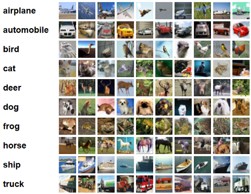
For training a model, we’ll use a basic Convolutional Neural Network (CNN) based on the Keras examples, but using the tf.Keras API rather than the separate reference implementation of Keras. We’ll train the CNN to classify images using the CIFAR-10 dataset, a well-known computer vision dataset. It consists of 60,000 32x32 images belonging to 10 different classes, with 6,000 images per class. Here is a graphic of the classes in the dataset, as well as 10 random images from each:

Setup

We’ll begin with some necessary imports, and get an Amazon SageMaker session to help perform certain tasks, as well as an IAM role with the necessary permissions.

%matplotlib inline
import numpy as np
import os
import sagemaker
from sagemaker import get_execution_role

sagemaker_session = sagemaker.Session()
role = get_execution_role()

bucket = sagemaker_session.default_bucket()
prefix = 'sagemaker/DEMO-tf-batch-inference-script'
print('Bucket:\n{}'.format(bucket))

Now we’ll run a script that fetches the dataset and converts it to the TFRecord format, which is convenient and often more performant for training models in TensorFlow.

!python generate_cifar10_tfrecords.py --data-dir ./data

For Amazon SageMaker hosted training on a cluster separate from this notebook instance, training data must be stored in Amazon S3, so we’ll upload the data to S3 now.

inputs = sagemaker_session.upload_data(path='data', key_prefix='data/DEMO-batch-cifar10-tf')
display(inputs)

Distributed training with Horovod

Although batch inference is the focus of this notebook, to begin we need a trained model. Sometimes it makes sense to perform training on a single machine. For large datasets, however, it may be necessary to perform distributed training on a cluster of multiple machines. In fact, it may be not only faster but cheaper to do distributed training on several machines rather than one machine. Fortunately, Amazon SageMaker makes it easy to run distributed training without having to manage cluster setup and tear down. Distributed training can be done using methods such as parameter servers or Ring-AllReduce with Horovod, an open source distributed training framework for TensorFlow, Keras, PyTorch, and MXNet.

For this notebook we’ll use Amazon SageMaker Script Mode to set up a Horovod-based training job. In Script Mode, your training job uses Amazon SageMaker’s prebuilt TensorFlow containers with TensorFlow training scripts similar to those you would use outside SageMaker. A major advantage of Script Mode is that only a few lines of code are necessary to use Horovod for distributed training with the tf.keras API. For details, see the train.py script included with this notebook; the changes primarily relate to:

• importing Horovod.

• initializing Horovod.

• configuring GPU options and setting a Keras/tf.session with those options.

Horovod is only available with TensorFlow version 1.12 or newer in Script Mode.

Once we have a training script, the next step is to set up an Amazon SageMaker TensorFlow Estimator object with the details of the training job. It is very similar to an Estimator for training on a single machine, except we specify a distributions parameter describing Horovod attributes such as the number of process per host, which is set here to the number of GPUs per machine. Beyond these few simple parameters and the few lines of code in the training script, there is nothing else you need to do to use distributed training with Horovod; Amazon SageMaker handles the heavy lifting for you and manages the underlying cluster setup.

from sagemaker.tensorflow import TensorFlow

hvd_instance_type = 'ml.p3.8xlarge'
hvd_processes_per_host = 4
hvd_instance_count = 2

distributions = {'mpi': {
                    'enabled': True,
                    'processes_per_host': hvd_processes_per_host,
                    'custom_mpi_options': '-verbose --NCCL_DEBUG=INFO -x OMPI_MCA_btl_vader_single_copy_mechanism=none'
                        }
                }
hyperparameters = {'epochs': 60, 'batch-size' : 256}

estimator_hvd = TensorFlow(base_job_name='dist-cifar10-tf',
                       source_dir='code',
                       entry_point='train.py',
                       role=role,
                       framework_version='1.13',
                       py_version='py3',
                       hyperparameters=hyperparameters,
                       train_instance_count=hvd_instance_count,
                       train_instance_type=hvd_instance_type,
                       tags = [{'Key' : 'Project', 'Value' : 'cifar10'},{'Key' : 'TensorBoard', 'Value' : 'dist'}],
                       distributions=distributions)

Now we can call the fit method of the Estimator object to start training. After training completes, the tf.keras model will be saved in the SavedModel .pb format so it can be served by a TensorFlow Serving container. Note that the model is only saved by the the master, rank = 0 process (disregard any warnings about the model not being saved by all the processes).

remote_inputs = {'train' : inputs+'/train', 'validation' : inputs+'/validation', 'eval' : inputs+'/eval'}
estimator_hvd.fit(remote_inputs)

Batch Transform with TFS pre/post-processing scripts

Amazon SageMaker lets you deploy a model to an endpoint for real-time inferences, or create a Transform Job for offline inference. If a use case does not require individual predictions in near real-time, an Amazon SageMaker Batch Transform job is likely a better alternative. Although hosted endpoints also can be used for pseudo-batch prediction, the process is more involved than using the alternative Batch Transform, which is designed for large-scale, asynchronous batch inference.

A typical problem in working with batch inference is how to convert data into tensors that can be input to the model. For example, image data in .png or .jpg format cannot be directly input to a model, but rather must be converted first. Additionally, sometimes other preprocessing of the data must be performed, such as resizing. The Amazon SageMaker TFS container provides functionality for doing this efficiently.

Pre/post-postprocessing inference script

The TFS container in Amazon SageMaker by default uses the REST API to serve prediction requests. This requires the input data to be converted to JSON format. One way to do this is to create a Docker container to do the conversion, then create an overall Amazon SageMaker model that links the conversion container to the TensorFlow Serving container with the model. This is known as an Amazon SageMaker Inference Pipeline, as demonstrated in another sample notebook.

However, as a more convenient alternative for many use cases, the Amazon SageMaker TFS container provides a data pre/post-processing script feature that allows you to simply supply a data transformation script. Using such a script, there is no need to build containers or directly work with Docker. The simplest form of a script must only (1) implement an input_handler and output_handler interface, as shown in the code below, (2) be named inference.py, and (3) be placed in a /code directory.

!cat ./code/inference.py

On the input preprocessing side, the code takes an image read from Amazon S3 and converts it to the required TFS REST API input format. On the output postprocessing side, the script simply passes through the predictions in the standard TFS format without modifying them. Alternatively, we could have just returned a class label for the class with the highest score, or performed other postprocessing that would be helpful to the application consuming the predictions.

Requirements.txt

Besides an inference.py script implementing the handler interface, it also may be necessary to supply a requirements.txt file to ensure any necessary dependencies are installed in the container along with the script. For this script, in addition to the Python standard libraries we need the Pillow and Numpy libraries.

!cat ./code/requirements.txt

Run a Batch Transform job

Next, we’ll run a Batch Transform job using our data processing script and GPU-based Amazon SageMaker Model. More specifically, we’ll perform inference on a cluster of two instances. The objects in the S3 path will be distributed between the two instances. In this example, our input can’t be split by newline characters and batched together, so the cluster will receive one HTTP request per serialized image.

The code below creates a SageMaker Model entity that will be used for Batch inference, and runs a Transform Job using that Model. The Model contains a reference to the TFS container, the TensorFlow SavedModel we trained above, the pre- and post-processing script, and the requirements.txt file.

For improved performance, we’ll set the max_concurrent_transforms and max_payload parameters of the Transformer object, which control the maximum number of parallel requests that can be sent to each instance in a transform job and the maximum size of each request body.

When performing inference on entire, unsplit S3 objects, it is recommended that you set max_payload to be slightly larger than the largest S3 object in your dataset, and that you experiment with the max_concurrent_transforms parameter in powers of two to find a value that maximizes throughput for your model.

from sagemaker.tensorflow.serving import Model

tensorflow_serving_model = Model(model_data=estimator_hvd.model_data,
                                 role=role,
                                 framework_version='1.13',
                                 sagemaker_session=sagemaker_session)

input_data_path='s3://sagemaker-sample-data-{}/tensorflow/cifar10/images/png'.format(sagemaker_session.boto_region_name)
output_data_path='s3://{}/{}/{}'.format(bucket, prefix, 'batch-predictions')
batch_instance_count=2
batch_instance_type = 'ml.p3.2xlarge'
concurrency=32
max_payload_in_mb=1

transformer = tensorflow_serving_model.transformer(
    instance_count=batch_instance_count,
    instance_type=batch_instance_type,
    max_concurrent_transforms=concurrency,
    max_payload=max_payload_in_mb,
    output_path=output_data_path
)

transformer.transform(data=input_data_path, content_type='application/x-image')
transformer.wait()

Inspect Batch Transform output

Finally, we can inspect the output files of our Batch Transform job to see the predictions. First we’ll download the prediction files locally, then extract the predictions from them.

!aws s3 cp --quiet --recursive $transformer.output_path ./batch_predictions

import json
import re

total = 0
correct = 0
predicted = []
actual = []
labels = ['airplane','automobile','bird','cat','deer','dog','frog','horse','ship','truck']
for entry in os.scandir('batch_predictions'):
    try:
        if entry.is_file() and entry.name.endswith("out"):
            with open(entry, 'r') as f:
                jstr = json.load(f)
                results = [float('%.3f'%(item)) for sublist in jstr['predictions'] for item in sublist]
                class_index = np.argmax(np.array(results))
                predicted_label = labels[class_index]
                predicted.append(predicted_label)
                actual_label = re.search('([a-zA-Z]+).png.out', entry.name).group(1)
                actual.append(actual_label)
                is_correct = (predicted_label in entry.name) or False
                if is_correct:
                    correct += 1
                total += 1
    except Exception as e:
        print(e)
        continue

Let’s calculate the accuracy of the predictions.

print('Out of {} total images, accurate predictions were returned for {}'.format(total, correct))
accuracy = correct / total
print('Accuracy is {:.1%}'.format(accuracy))

The accuracy from the batch transform job on 10000 test images never seen during training is fairly close to the accuracy achieved during training on the validation set. This is an indication that the model is not overfitting and should generalize fairly well to other unseen data.

Next we’ll plot a confusion matrix, which is a tool for visualizing the performance of a multiclass model. It has entries for all possible combinations of correct and incorrect predictions, and shows how often each one was made by our model. Ours will be row-normalized: each row sums to one, so that entries along the diagonal correspond to recall.

import pandas as pd
import seaborn as sns

confusion_matrix = pd.crosstab(pd.Series(actual), pd.Series(predicted), rownames=['Actuals'], colnames=['Predictions'], normalize='index')
sns.heatmap(confusion_matrix, annot=True, fmt='.2f', cmap="YlGnBu").set_title('Confusion Matrix')

If our model had 100% accuracy, and therefore 100% recall in every class, then all of the predictions would fall along the diagonal of the confusion matrix. Here our model definitely is not 100% accurate, but manages to achieve good recall for most of the classes, though it performs worse for some classes.

Model Deployment with Amazon Elastic Inference

Amazon SageMaker also lets you deploy a TensorFlow Serving model to a hosted Endpoint for real-time inference. The processes for setting up hosted endpoints and Batch Transform jobs have significant differences, as we will see. Additionally, we will discuss why and how to use Amazon Elastic Inference with the hosted endpoint.

Deploying the Model

When considering the overall cost of a machine learning workload, inference often is the largest part, up to 90% of the total. If a GPU instance type is used for real time inference, it typically is not fully utilized because, unlike training, real time inference does not involve continuously inputting large batches of data to the model. Elastic Inference provides GPU acceleration suited for inference, allowing you to add inference acceleration to a hosted endpoint for a fraction of the cost of using a full GPU instance.

Instead of a Transformer object, we’ll instantiate a Predictor object now. The deploy method of the Estimator object instantiates a Predictor object representing an endpoint which serves prediction requests in near real time. To utilize Elastic Inference with the SageMaker TFS container, simply provide an accelerator_type parameter, which determines the type of accelerator that is attached to your endpoint. Refer to the Inference Acceleration section of the instance types chart for a listing of the supported types of accelerators.

Here we’ll use a general purpose CPU compute instance type along with an Elastic Inference accelerator: together they are much cheaper than the smallest P3 GPU instance type.

predictor = estimator_hvd.deploy(initial_instance_count=1,
                                  instance_type='ml.m5.xlarge',
                                  accelerator_type='ml.eia1.medium')

Real time inference

Now that we have a Predictor object wrapping a real time Amazon SageMaker hosted endpoint, we’ll define the label names and look at a sample of 10 images, one from each class.

from IPython.display import Image, display

images = []
for entry in os.scandir('sample-img'):
    if entry.is_file() and entry.name.endswith("png"):
        images.append('sample-img/' + entry.name)

for image in images:
    display(Image(image))

Next, we’ll modify some properties of the Predictor object created by the deploy method call above. The TFS container in Amazon SageMaker by default uses the TFS REST API, which requires requests in a specific JSON format. However, for many real time use cases involving image data it is more convenient to have the client application send the image data directly to an endpoint for predictions, without converting and preprocessing it on the client side.

Fortunately, our endpoint includes the same pre/post-processing script used in the Batch Transform section of this notebook because the same model artifact is used in both cases. This model artifact includes the same inference.py script. With this preprocessing script in place, we just specify the Predictor’s content type as application/x-image and override the default serializer. Then we can simply provide the raw .png image bytes to the Predictor.

predictor.content_type = 'application/x-image'
predictor.serializer = None

labels = ['airplane','automobile','bird','cat','deer','dog','frog','horse','ship','truck']

def get_prediction(file_path):

    with open(file_path, "rb") as image:
        f = image.read()
    b = bytearray(f)
    return labels[np.argmax(predictor.predict(b)['predictions'], axis=1)[0]]

predictions = [get_prediction(image) for image in images]
print(predictions)

Extensions

Although we did not demonstrate them in this notebook, Amazon SageMaker provides additional ways to make distributed training more efficient for very large datasets: - VPC training: performing Horovod training inside a VPC improves the network latency between nodes, leading to higher performance and stability of Horovod training jobs.

• Pipe Mode: using Pipe Mode reduces startup and training times. Pipe Mode streams training data from S3 as a Linux FIFO directly to the algorithm, without saving to disk. For a small dataset such as CIFAR-10, Pipe Mode does not provide any advantage, but for very large datasets where training is I/O bound rather than CPU/GPU bound, Pipe Mode can substantially reduce startup and training times.

Cleanup

To avoid incurring charges due to a stray endpoint, delete the Amazon SageMaker endpoint if you no longer need it:

sagemaker_session.delete_endpoint(predictor.endpoint)